Set Operations in R

R can perform different operations in sets, such as union, intersection, asymmetric difference of two sets, etc. Specifically, the following operations are available in R for set operations.

Operator	Usage	Definition
union	union(x, y)	Union of sets x and y
intersect	intersect(x, y)	Intersection of sets x and y
setdiff	setdiff(x, y)	Asymmetric difference between sets x and y (Elements in x but not in y)
setequal	setequal(x, y)	If sets x and y have the same elements
is.element	is.element(el, set)	If el is an element of set

Examples:

> x <- c(sort(sample(1:20, 9)),NA)

> y <- c(sort(sample(3:23, 7)),NA)

> x

[1]  1  3  5  8 11 17 18 19 20 NA

> y

[1]  7 11 15 16 17 19 22 NA

> union(x, y)

[1]  1  3  5  8 11 17 18 19 20 NA  7 15 16 22

> intersect(x, y)

[1] 11 17 19 NA
> setdiff(x, y)

[1]  1  3  5  8 18 20

> setdiff(y, x)

[1]  7 15 16 22

> setequal(x, y)

[1] FALSE

Note that each of union, intersect, setdiff and setequal will discard any duplicated values in the arguments. Look at the following example:

> x

[1]  1  3  5  8 11 17 18 19 20 NA

> x2 <- c(x, 1, 3, 5, 8)

> x2

[1]  1  3  5  8 11 17 18 19 20 NA  1  3  5  8

> setdiff(x, y)

[1]  1  3  5  8 18 20

> setdiff(x2, y)

[1]  1  3  5  8 18 20

> setequal(x, x2)

[1] TRUE

Although x and x2 have different length, they have the same UNIQUE elements so setequal(x, x2) returns a TRUE value.

is.element(x, y) is identical to x %in% y which is already discussed here. The return value of is.element is a vector of TRUE and FALSE with the same length as x, which indicates whether each element of x is an element of y or not.

> is.element(x, y)  # vector of length 10

[1] FALSE FALSE FALSE FALSE  TRUE  TRUE FALSE  TRUE FALSE  TRUE

> is.element(y, x)  # vector of length 8

[1] FALSE  TRUE FALSE FALSE  TRUE  TRUE FALSE  TRUE

Running time in R

In R, proc.time determines how much real and CPU time (in seconds) the currently running R process has already taken. proc.time returns five elements for backwards compatibility, but prints a named vector of length 3. The first two entries are the total user and system CPU times of the current R process and any child processes on which it has waited, and the third entry is the ‘real’ elapsed time since the process was started. system.time(expr) is used for timing a valid R expression which calls the function proc.time, evaluates expr, and then calls proc.time once more, returning the difference between the two proc.time calls. For example,

> ptm <- proc.time()

> for (i in 1:10000) x <- rnorm(1000)

> proc.time() - ptm

   user  system elapsed

   2.10    0.01    2.14
> system.time(for (i in 1:10000) x <- rnorm(1000))
   user  system elapsed
   2.01    0.00    2.06 

The definition of 'user' and 'system' times is from your OS. Typically it is something like

The 'user time' is the CPU time charged for the execution of user instructions of the calling process. The 'system time' is the CPU time charged for execution by the system on behalf of the calling process.

proc.time/system.time can be used to compare the running speed of different methods doing the same job. For example, we want to find out the maximum of a vector of 10000000 randomly generated Uniform[0,1] random variables.

> x<-runif(10000000)

> system.time(max(x))

   user  system elapsed

   0.05    0.00    0.05

> pc <- proc.time()

> cmax <- x[1]

> for (i in 2:10000000)

+ {

+   if(x[i] > cmax) cmax <- x[i]

+ }

> proc.time() - pc

   user  system elapsed

  16.88    0.11   18.21

We can see that there is a huge difference in running time between the two methods (0.05 seconds versus 18.21 seconds). Do not 'grow' data sets in loops or recursive function calls. Use R built-in functions whenever possible.

Complex numbers in R

We sometimes encounter the situations of using complex numbers in our computation. For example, the square root of -1 can be denoted as 1*i. Complex numbers are implemented in the "base" package, it’s very easy to work with them. To construct a complex number x + iy, you use complex and specify its real and imaginary components explicitly as follows:

> x <- 2

> y <- 3

> z1 <- complex(real = x, imaginary = y)

> z1

[1] 2+3i

You can convert other objects to class "complex" using as.complex and test if an object is complex with is.comple

> z2 <- as.complex(-5)
> z2
[1] -5+0i
> is.complex(z2)
[1] TRUE

There are five basic mathematical operations that works on complex numbers, Re, Im, Mod, Arg, and Conj. First, you may want to extract the real and imaginary components of a complex number. You can do this using Re and Im, respectively. You can also find the modulus and complex argument of a complex number with Mod and Arg. Finally, you can take the complex conjugate of a complex number with the help of Conj.

> z3 <- complex(real = 1.3, imaginary = 6) 

> z3

[1] 1.3+6i

> Re(z3)

[1] 1.3

> Im(z3)

[1] 6

> Mod(z3)

[1] 6.139218

> Arg(z3)

[1] 1.357428

> Conj(z3)

[1] 1.3-6i

Special symbols and math formulas in R

Sometimes one wants to put special symbols, such as Greek letters and superscripts on the plots. In R we can use function expression() to do this job.

> xlabel <- expression(paste(Delta, italic(s), sep = ""))

> ylabel <- expression(alpha[1] * " in (kg)"^2)

> plotname <- expression(sin * (beta))

> plot(rnorm(50), rnorm(50), xlab = xlabel, ylab = ylabel, main = plotname, xlim = c(-pi, pi), ylim = c(-3, 3), axes = FALSE)

> axis(1, at = c(-pi, -pi/2, 0, pi/2, pi), labels = expression(-pi, -pi/2, 0, pi/2, pi))

> axis(2)
> box()

> text(-pi/2, -2, expression(hat(beta) == (X^t * X)^{-1} * X^t * y))

> text(pi/2, 2, expression(paste(frac(1, sigma*sqrt(2*pi)), exp*(frac(-(x-mu)^2, 2*sigma^2)), sep = "")), cex = 1.5)

If you want to know more about expression and putting math symbols on the plot, run the following demos in R.

> demo(plotmath)

Find all the matches between two vectors using %in% in R

Suppose you want to know all of the matches between one character vector and another, you can do that with the help of which and %in% in R. For example,

> allclasses <- c("physics", "chemistry", "statistics", "mathematics", "biology", "history", "english")

> registered <- c("physics", "mathematics", "history")

> which(allclasses %in% registered)
[1] 1 4 6

This also works with numeric vectors. For example, a numeric set B is a subset of A, and you want to select all those elements that are included in A but not B. You can do the following:

> A <- c(1, 2, 3, 5, 8, 13, 21, 34, 55, 89)

> B <- c(1, 5, 21, 89)

> A[!(A %in% B)]

[1]  2  3  8 13 34 55

Export to multiple-sheet xls file in R

It's easy to export a data frame or table to .csv file in R. However, sometimes one want to save to a .xls file directly. You can certainly first export to a .csv file and convert it to a .xls file in Microsoft Excel, but the following R codes can do this job directly with ability to save a multiple-sheet .xls file.

> install.packages("RODBC")

> library(RODBC)

> save2excel <- function(x, tname) sqlSave(xlsFile, x, tablename = tname, rownames = FALSE, addPK = T)

> xlsFile <- odbcConnectExcel("C:\\Temp\\test.xls", readOnly = FALSE)

> temp1 <- data.frame(x = rnorm(100), y = rnorm(100))

> temp2 <- data.frame(x = rnorm(100), y = rnorm(100))

> save2excel(temp1, "test1") # Here test is the name of current sheet

> save2excel(temp2, "test2")

> odbcCloseAll()

Value of last evaluated expression in R

R saves the value of last evaluated expression in a variable called .Last.value. You can directly use this variable instead of running the last expression again.

For example:

> x <- 1:10

> x^2

[1] 1 4 9 16 25 36 49 64 81 100

> y <- .Last.value

> y

[1] 1 4 9 16 25 36 49 64 81 100

Remove inner margins in R plots

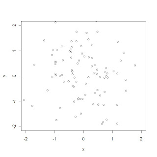
You may notice that xlim and ylim options in R plots do not make the horizontal and vertical axes start and end at your specified values. Instead, by default the specified ranges are enlarged by 6%, so that the specified values do not lie at the very edges of the plot region. This is appropriate for most types of plot, but sometimes we want the specified limits to lie at the edges of the plot window. This can be specified separately for each axis using the arguments xaxs and yaxs. Please refer to the following example and pay attention to the difference of corners in the two plots.

Here is the help document on xaxs and yaxs in R.

xaxs

The style of axis interval calculation to be used for the x-axis. Possible values are "r", "i", "e", "s", "d". The styles are generally controlled by the range of data or xlim, if given. Style "r" (regular) first extends the data range by 4 percent at each end and then finds an axis with pretty labels that fits within the extended range. Style "i" (internal) just finds an axis with pretty labels that fits within the original data range. Style "s" (standard) finds an axis with pretty labels within which the original data range fits. Style "e" (extended) is like style "s", except that it is also ensures that there is room for plotting symbols within the bounding box. Style "d" (direct) specifies that the current axis should be used on subsequent plots. (Only "r" and "i" styles are currently implemented)

> x <- rnorm(100)

> y <- rnorm(x)

> plot(x, y, xlim = c(-2, 2), ylim = c(-2, 2))

> plot(x, y, xlim = c(-2, 2), ylim = c(-2, 2), xaxs = "i", yaxs = "i")